Before calculating a cable run, identify its current path, resistance basis, and load state. One-way route length, total conductor length, and complete loop resistance are different inputs. Choosing the right values prevents a return conductor from being counted twice or a shared segment from carrying the wrong current.
Choose the electrical model from the return path
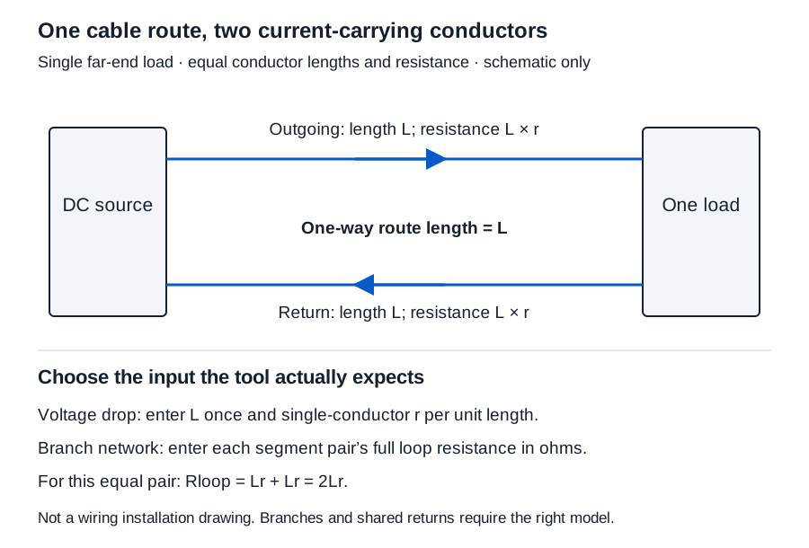
The two-wire voltage-drop calculator models one far-end constant-current load with equal outgoing and return conductors. Enter one-way route length and resistance per unit length of one conductor. The calculation includes the equal return.
The branch-network calculator models a rooted tree with independent outgoing/return segment pairs. Enter each pair’s complete loop resistance in ohms, along with its local load current. Parent 0 is the source; another parent must refer to an earlier node. Each upstream segment carries its downstream currents.
| Tool | Length input | Resistance input | Return treatment |
|---|---|---|---|
| Two-wire voltage drop | One-way ft or m | Ω/1000 ft or Ω/km for one conductor | Equal return included by the tool |
| Maximum one-way length | Solved output | Same per-conductor basis | Equal return included |
| Branch network | No separate route-length field | Complete segment-pair Ω | Already contained in the supplied resistance |
| Wire resistance | One-way ft or m | Applicable resistivity and conductive area | Select single conductor or equal loop explicitly |
Work a two-wire run without doubling its length
Use hypothetical 24 V source, 1 A load, 100 ft one-way route, and 10 Ω/1000 ft per conductor. These resistance and current values are examples, not wire-gauge recommendations.
- Select voltage-drop mode in the two-wire tool.
- Enter source
24, current1, and one-way distance100with feet selected. - Enter resistance
10with Ω/1000 ft selected. - Calculate and retain the load state and resistance source with the output.
One conductor = (100/1000) × 10 = 1 Ω
Loop = 1 + 1 = 2.000 Ω
Drop = I × Rloop = 1 × 2 = 2.000 V
Load-end voltage = 24 − 2 = 22.000 V
Loss = I²Rloop = 1² × 2 = 2.000 W
Drop percentage is 100 × 2/24 = 25/3%, displayed 8.333%. Source voltage and resistance must be positive; current and distance may explicitly be zero in this forward model. Length and resistance-unit controls are independent.
Entering 30.48 m instead of 100 ft gives the same physical result because 1 ft = 0.3048 m exactly. Entering 200 ft would count the return twice and incorrectly produce 20 V for this case.
Reuse the loop value only in a model that expects it
For a single branch-network node, enter 0,2,1: source parent 0, complete pair resistance 2 Ω, and local load 1 A. With a 24 V source, its voltage is again 22.000 V. Do not double that 2 Ω input.
For a two-node illustration, enter 0,2,0 then 1,1,1. The first segment carries the downstream 1 A and drops 2 V. The second drops 1 V, leaving 21.000 V at node 2. An unloaded upstream node still carries downstream current. Up to 30 nodes are supported; zero local current or segment resistance must be explicit.
These calculations follow series resistance and IR drop. Compare the result with actual device requirements separately. A nonpositive load-end voltage means the stated-current operating assumption is unusable there; it does not predict reverse polarity caused by passive wire.
Solve a voltage boundary without treating it as a cutting instruction
Select maximum one-way length mode and supply a documented minimum device voltage. With the same 24 V, 1 A, and 10 Ω/1000 ft, an illustrative 22 V minimum gives:
r = 10/1000 = 0.01 Ω/ft per conductor
Lmax = (Vsource − Vminimum)/(2Ir)
Lmax = (24 − 22)/(2 × 1 × 0.01) = 100.000 ft = 30.480 m
Minimum voltage, current, and resistance must be positive; minimum voltage cannot exceed the source. This is the exact boundary of the stated uniform model. Source variation, connections, temperature, and equipment behavior require separate design consideration.
If estimating resistance from material data, retain conductive area, applicable resistivity, reference temperature, and any justified temperature coefficient. Bulk arithmetic does not establish finished-cable performance.
Compare candidate conductors on the same basis
The two-wire tool’s candidate comparison applies the same source voltage, minimum device voltage, load current, and one-way length to each supplied conductor resistance. Keep a product/source record for every candidate and state one common temperature and condition basis. AWG in a label does not select resistance data or establish ampacity.
With hypothetical 24 V, 20 V minimum, 1 A, and 100 ft, single-conductor resistances of 10, 20, and 25 Ω/1000 ft leave 22, 20, and 19 V. Their voltage margins are +2, 0, and −1 V. Equality has no modeled margin; even a tiny unrounded deficit must remain below the threshold when the display rounds to 20.000 V. Retain the source data and exact margin for review, then check actual equipment and installation requirements separately.
Survey pathway geometry separately
The pathway occupancy calculator uses clear circular internal diameter and each cable’s actual outside diameter and quantity. For four hypothetical 5 mm cables in a 20 mm clear pathway:
Area ratio = 4 × 5²/20² × 100 = 25.000%
π cancels. This is area accounting, not a packing solution, permitted fill, pulling clearance, or ampacity result. Trade size cannot substitute for clear internal diameter. A conduit offset calculation concerns bender marks; those marks do not establish finished cable length.
Keep the run definition with the result
Record construction, temperature, typical/maximum resistance basis, units, datasheet revision, current state, route, and return topology. Use the resistance record to preserve the single-conductor versus loop distinction. Results use original arithmetic before three-decimal display rounding. Obtain missing data before relying on a result, then separately verify equipment voltage, protection, physical installation requirements, and applicable rules.